How to Make Excel Pivot Table

Pivot tables in Excel are a powerful tool for summarising, analysing, and presenting data. They allow you to quickly extract meaningful insights from large datasets.In this article we will learn pivot tables in excel.

How to make excel pivot tables:

To create a pivot table in excel follow below given steps.

1 From Insert Panel Click On Insert Pivot table Button

2 Click On Pivot Table a window will Pop up as shown below

3 Click On New Worksheet or Existing Worksheet Where You Want To Insert Pivot table and Then Click Ok.

4 Then Put The Right Hand Shown Element In Row Labels and In Values Section To Make Pivot Table As shown Below

5 Pivot Table Is Ready. Now You Can Select All By Pressing (CTRL+A) and Copy (CTRL+C) and Special Paste(ALT+H+V+V) Data To remove Formula.

So it is how you can make Pivot Table In excel which is very commonly used in making reports.

Distinct Count in Pivot Tables in Excel:

To take unique count we can take distinct count in pivot table.to begin with

1. We have to tick add this data to data model as shown in image below then make click ok and make pivot table.

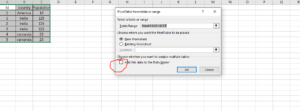
        2.Then right click on field enter in values then click on value field setting from it select distinct count and click                  ok.

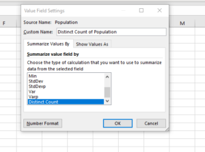
Now it will count unique values.

How to Group dates in Pivot Tables in Excel:

We can group dates in pivot table by using “Group Selection” button in excel.We can group monthly,day-wise,year-wise etc.

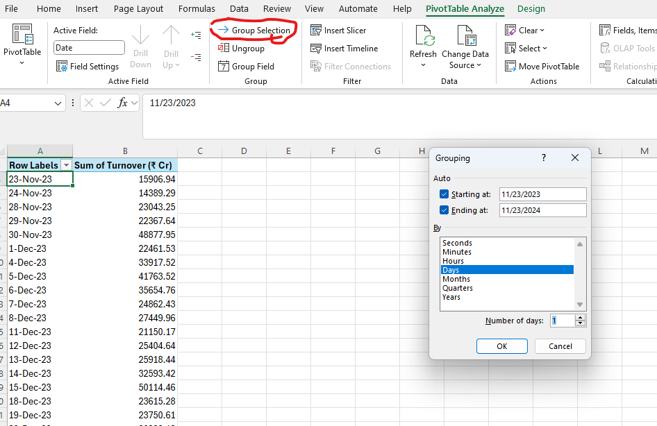
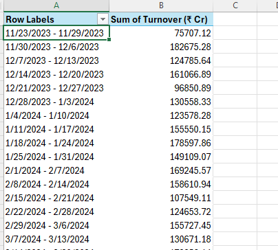
As shown above first you have to click on  Pivot table analyse.Then you have to click on option “Group Selection”.A window will pop up showing seconds,month,hours,days,quarters,years.Form here you can select year to group by yearly or if you want to group by weekly just click on days and then in number of days put 7 and click ok dates and all data will be grouped by weekly as shown below

Excel Pivot table Sort data:

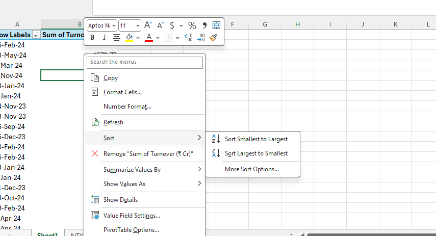
In above we have learnt how to make excel pivot table To Sort data in pivot table.First we have to right click on table then from it click on sort under it  two option will come sort smallest to largest and sort largest two smallest.From here we can sort values as required.