INDEX in Excel
In Excel, the INDEX function is used to retrieve a value from within a specified range based on row and column numbers.
Syntax of the INDEX Function
INDEX(array, row_num, [column_num])
- array: This is the range of cells or array from which you want to retrieve data.
row_num: This specifies the row number in the array from which to retrieve data.column_num(optional): This specifies the column number in the array from which to retrieve data. If omitted, column_num defaults to the same value as row_num.
Examples of Using INDEX
Assume you have the following data in cells A1 to J22
| A | B | C | D | E | F | G | H | I | J |
| 0 | 0 | 0 | 0 | 0 | 0 | 0 | 0 | 0 | 1 |
| 1 | 0 | 0 | 0 | 0 | 0 | 0 | 1 | 0 | 0 |
| 0 | 0 | 0 | 0 | 0 | 0 | 0 | 1 | 1 | 0 |
| 0 | 0 | 0 | 0 | 0 | 0 | 0 | 1 | 0 | 1 |
| 0 | 0 | 0 | 0 | 0 | 0 | 0 | 0 | 1 | 0 |
| 0 | 0 | 0 | 0 | 0 | 0 | 0 | 1 | 0 | 1 |
| 0 | 0 | 0 | 0 | 0 | 0 | 0 | 0 | 1 | 0 |
| 0 | 0 | 0 | 0 | 0 | 0 | 1 | 0 | 0 | 0 |
| 0 | 0 | 0 | 0 | 0 | 0 | 1 | 0 | 0 | 0 |
| 0 | 0 | 0 | 0 | 0 | 0 | 1 | 0 | 0 | 0 |
| 0 | 0 | 0 | 0 | 0 | 0 | 1 | 1 | 0 | 0 |
| 0 | 0 | 0 | 0 | 0 | 0 | 1 | 0 | 0 | 0 |
| 0 | 1 | 0 | 0 | 0 | 0 | 1 | 0 | 0 | 0 |
| 0 | 0 | 0 | 0 | 0 | 0 | 1 | 1 | 0 | 0 |
| 0 | 1 | 0 | 0 | 0 | 1 | 0 | 0 | 0 | 0 |
| 0 | 0 | 0 | 0 | 0 | 0 | 0 | 0 | 1 | 0 |
| 0 | 1 | 1 | 3 | 1 | 0 | 0 | 0 | 0 | 0 |
| 0 | 1 | 0 | 0 | 0 | 1 | 0 | 0 | 0 | 1 |
| 0 | 0 | 0 | 0 | 0 | 1 | 1 | 1 | 0 | 0 |
| 0 | 0 | 0 | 0 | 0 | 0 | 1 | 1 | 0 | 0 |
| 1 | 0 | 0 | 0 | 0 | 0 | 0 | 1 | 0 | 0 |
To retrieve the value in the 1 row of Column J (which is 1), you can use:
| =INDEX(A2:J22,1,10) |
MATCH in Excel
In Excel, the MATCH function is used to locate the position of a value in a range of cells. It’s particularly useful when you need to find the position of a specific item in a row, column, or even a one-dimensional array. Here’s how you can use the MATCH function effectively:
Syntax of the Match Function
MATCH(lookup_value, lookup_array, [match_type])
- lookup_value: This is the value you want to find within the lookup_array.
- lookup_array: This is the range of cells or an array where Excel searches for the lookup_value.
- match_type: This is an optional argument that specifies the type of match:
0(Exact match): Finds the first value exactly equal to lookup_value.1(Less than): Finds the largest value less than or equal to lookup_value. Thelookup_arraymust be in ascending order.-1(Greater than): Finds the smallest value greater than or equal to lookup_value. The lookup_array must be in descending order.
Examples of Using the MATCH Function
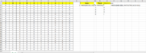
In Above table if we have to find index or position of value 1 (which is 10) then we will use this formula
| =MATCH(1,A2:J2,0) |
lookup_value is 1 what we are looking for.
lookup_array A2:J2 within which excel will search and Zero(0) for Exact Match.
MATCH formula will return first match of the occurrence
How to use Index and Match together in excel
If we have to find the column name where values is greater than zero .The we can use both index and match together a shown below
| =INDEX($A$1:$J$1,,MATCH(TRUE,A2:J2>0,0)) |

How to find 2nd,3rd and nth Match in Excel
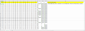
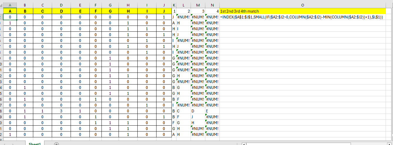
MATCH formula will return first match of the occurrence To find 2nd,3rd and nth occurrence in excel we have to use INDEX formula with SMALL,IF and COLUMN function in table.
| =INDEX($A$1:$J$1,SMALL(IF($A2:$J2>0,COLUMN($A2:$J2)-MIN(COLUMN($A2:$J2))+1),$L$1)) |

